Clicking on the Preview Statistics icon will open a window summarizing the statistics from your last fitting exercise. Clicking on the Export to Excel button at the bottom of this window will automatically write these results to your Excel workbook.  You can also generate an Excel or HTML report using  and  from the Fitting toolbar.

Details of and equations used in calculating fitting statistics are presented below.  The symbol y is any response that is being fitted, i and j refer to the ith data point in the jth series; superscript ex indicates the experimental measurement and _ij the standard deviation of the measurement error distribution for measurement ij.

A good source of additional information on fitting and optimization algorithms and theory is Numerical Recipes in Fortran, 2nd edition, by W.H. Press, S.A. Teukolsky, W.T. Vetterling and B.P. Flannery, Cambridge University Press, 1992.

Variance-covariance matrix

The covariance matrix is calculated from the inverse of the second derivative matrix (matrix of second derivatives of the SSQ with respect to the parameters):

                                

       

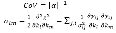
This is evaluated by forward differencing. If weighted or unweighted SSQ are used, the final SSQ value is scaled with back-calculated errors so that it equals the number of degrees of freedom.

 

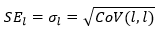
Standard errors on fitted parameters
The standard error on each fitted parameter is calculated from the covariance matrix (the square root of the diagonal of the covariance matrix):

                                         

 

Correlation matrix
The correlation matrix is a normalized form of the covariance matrix.

                                    

 

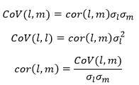
When two fitted parameters are highly correlated, the correlation coefficient may be 0.99 or more. This makes it difficult to fit values of these parameters with tight confidence intervals. This problem may be solved if for example it is possible to fit one parameter and its ratio to the other parameter.

 

Confidence intervals

Confidence intervals on fitted parameters are calculated from the covariance matrix:

                                                           

 

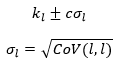
where c depends on the confidence level. For 90%, 95% and 99% confidence levels respectively the value of c is 1.65, 1.96 and 2.58.

t statistic

The t statistic is the ratio of the parameter value to its standard error. This gives an indication of whether the fitted value of the parameter is statistically significant. The value of the t-statistic is compared to a t distribution with N-p degrees of freedom (N is the number of data points and p is the number of parameters fitted).

For a statistically significant fit of a parameter, the following guidelines apply:

        90% confidence level t>1.68

        95% confidence level t>1.96

        99% confidence level t>2.58

The t-statistic is closely related to the confidence interval on the parameter estimate (the confidence interval is proportional to the standard error divided by the parameter value). A confidence interval above 100% is an indication that the fit is not statistically significant.

The t statistic, critical t value for 95% confidence and the probability for the t value are quoted for each parameter. The probability will be close to zero when the parameter value is statistically significant.

Coefficient of determination

This quantifies the amount of the variability in the data that is captured by the model. A value near 1 indicates a good representation of the data by the model.

Consistent with convention for linear regression of a model with an intercept, the denominator includes subtraction by the average of the data:

                                    

                                 

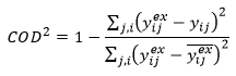
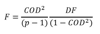
The coefficient of determination is related to the conventional F statistic calculated for linear regression with an intercept, as follows:

                            

 

Correlation coefficient, R²

This is very similar to coefficient of determination and again a value near 1 indicates a good representation of the data by the model.

Complementing the coefficient of determination above, R-squared is calculated for a model with no intercept and the denominator does not include subtraction by the average of the data: 

                             

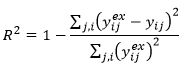
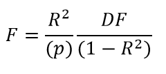
R-squared is related to the F statistic calculated by the Fitting window for models with no intercept, as follows:

                              

Degrees of freedom

The degrees of freedom is the number of selected data points minus the number of fitted parameters:

                                        

 

SSQ or Chi-squared

The choice of data weighting method determines whether SSQ_final (which is directly proportional to ²) or ² is reported. In all cases:

                                      

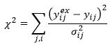
The choice of data weighting method affects only the standard deviation of the measurement error used in the denominator. SSQ_final is reported with weighted SSQ and unweighted SSQ and Chi-squared is reported with user-defined errors. The standard deviations used in all methods to obtain ² are given in the Excel and web reports, alongside each data point in the table of residuals.

SSQ_final is calculated from:

                                      

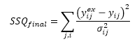
with, in the case of weighted SSQ, for all point in the jth series:

                                      

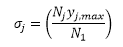
and, in the case of unweighted SSQ, with _ij =1.

 

Log-likelihood

Dynochem’s parameter fitting algorithms all use ‘maximum likelihood’ as the objective function that is to be maximized by changing model fitted parameters. Additional details on this approach are available in this KB article. 

In general, it is more convenient to work with the log of the likelihood and this statistic is reported for all data weighting methods:

                              

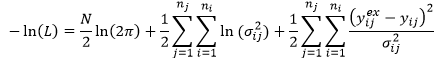
Maximum likelihood (L) corresponds with minimum negative log-likelihood -ln(L). Therefore lower values of the reported –ln(L) are better.

The first term depends only on the number of data points; the second term depends only on the standard deviations of the measurement error distribution, which is assumed to be a normal distribution; the third term is half of the ² statistic. 

During the fitting process (iterations), only the third term changes as the fitted parameter values are changed. When user-defined errors are provided, these are used directly to calculate log likelihood. When weighted SSQ or unweighted SSQ are used, back-calculated errors are used after scaling so that ²=DF=N-p.

It is possible with user-defined errors to estimate by how much the errors should be scaled in order to increase likelihood. This will in general also result in ²≈DF and a goodness of fit score in the range where residuals and measurement errors overlap. See this KB article for more information.

A good source of additional information on fitting and optimization algorithms and theory is Numerical Recipes in Fortran, 2nd edition, by W.H. Press, S.A. Teukolsky, W.T. Vetterling and B.P. Flannery, Cambridge University Press, 1992.

       

Goodness of fit

An independent goodness of fit (Q) assessment is possible if user defined errors have been supplied by the user (see data weighting method). This compares the chi-squared value with the value expected from a cumulative chi-squared distribution:

                                                  

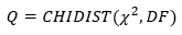
If the value of chi-squared is near to the number of degrees of freedom (DF=N-p), then a Q score of about 0.5 is obtained. This goodness of fit statistic, Q, assumes that user-defined errors are normally distributed.

Both the default data weighting method of weighted SSQ and the alternative unweighted SSQ back-calculate the standard deviation of the measurement error distribution that would produce a goodness of fit score of Q≈ 0.5. That score corresponds with a good level of overlap between model residuals and experimental errors. The ‘average error value’ resulting from this analysis is reported with the goodness of fit score; individual errors for each data point are included in the Excel and web reports beside the table of residuals.

 

Average error

When the data weighting method is weighted SSQ or unweighted SSQ, Dynochem reports as 'average error' the arithmetic mean of the back-calculated errors for each series that correspond with good overlap between experimental errors and model residuals. This summary value may be useful when all data series represent the same response (e.g. heat flow, Qr, or Substrate concentration).

 

Notes

The Notes section contains comments on the goodness of fit and how this relates to the relationship between experimental errors and model residuals. 

The following notes are reported with the goodness of fit score to assist interpretation of Q values:

0.95 < Q ≤ 1	Residuals are smaller than experimental errors. Errors may be overestimated.
1E-3 ≤ Q ≤ 0.95	Residuals are similar to experimental errors.　Good fit if residuals are normally distributed.
-1 < Q < 1e-3	Residuals are greater than experimental errors. Model does not match data and/or residuals are not normally distributed and/or errors are underestimated.

 

F statistic

The F statistic is the ratio of the variation explained by the model to the variation unexplained by the model.

Consistent with the calculation of R-squared and the relationship between R-squared and F for a model without an intercept, the Fitting window calculates F using a numerator that does not include subtraction by the average of the data:

                                         

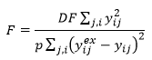
The F statistic is compared to an F distribution with p and DF degrees of freedom respectively. For example, when fitting 3 parameters to 20 data points, the value of F for a 95% confidence level is 19.16. This means that the F statistic calculated should be larger than this for statistical significance at the 95% confidence level. The probability reported with F will be close to zero when the model is statistically significant.

Notice that the number of parameters (p) appears in the denominator, indicating that doubling the number of parameters would approximately halve the F statistic. The F statistic can therefore be used to test the beneficial or otherwise effect of fitting more parameters. If the F statistic increases, the model has been improved by adding the parameters, but if F decreases then the model was not improved by adding the parameters.

 

Model selection criterion

The following model selection criterion can be used to compare the fit of two models to the same data, e.g. for model discrimination. This criterion is related to the Akaike Information Criterion (AKAIKE H (1976) An information criterion. Math. Sci. 14 (1) 5-9):

       

                                           

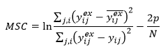
The numerator depends only on the experimental data and this term helps to scale MSC so that it does not depend on units of measure. The denominator is related to likelihood. The second term penalizes the MSC for inclusion of additional model fitted parameters. 

MSC can for example be used to compare fitting a two step reaction to data versus a single step reaction. A higher MSC suggests a better model.

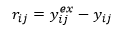
In order to simplify the appearance of the equations in this section on analysis of residuals, the following notation is used for residuals:

                                               

 

Mean absolute percentage deviation

This statistic is one measure of the average deviation between model predictions and measured values:

                                           

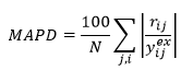
Lower values of MAPD indicate lower average percentage deviation between model and data.

 

Serial correlation of residuals

In a good model, residuals should be random and normally distributed. 

The Durbin-Watson statistic is used to calculate first order autocorrelation of residuals. This indicates whether there is likely to be a systematic trend in the residuals, indicating a possibly incorrect model.  This statistic is calculated using unweighted residuals for all responses.  We calculate a normalized value that ranges from -0.5 to 0.5:

                                              

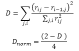
If no autocorrelation is present, D_norm=0.

 

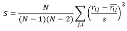
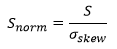
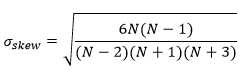
Normalized skewness of residuals

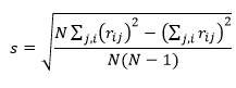
Skewness is a measure of the symmetry of the distribution of residuals:       

       

                                   

in which the sample standard deviation of residuals is:

                                  

A good model should have a skewness close to zero indicating that the unweighted residuals are normally distributed.  The skewness reported by Dynochem is normalized, so a skewness of greater than 1 (or less than -1) indicates somewhat non-normal behavior. Often, one or two outliers can significantly skew the distribution:

                                                         

where 

                               

 

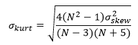
Normalized kurtosis of residuals

Like the skewness, the kurtosis measures the normality of the distribution of residuals. The reported kurtosis is normalized and values close to zero indicate a distribution close to the normal distribution:

                          

                                                                       

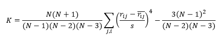
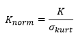
where

                                                           

A good reference for further reading on the above analysis of residuals and their normalization is the NIST website, especially Measures of Skewness and Kurtosis.